Omnis tempus datum - Cheminformatics basics - RDkit, regression models, similarity

Walkthrough on reading, visualizing, manipulating molecules and their properties using Pandas and RDKit for Cheminformatics-related tasks. In this file we will be primarly using SMILES to describe the molecules of choice.

What are SMILES?

Simplified molecular input line entry system (SMILES) is a form of line notation for describing the structure of chemical species using text strings. More details can be found here

Other resources:

Nice low-barrier intro to using some basic functions in RDkit: Xinhao Lin’s RDKit Cheatsheet, I’ve adopted some of the functions frrom that blog in here:
Rdkit Tutorial github
Patrick Walters’ Learning Cheminformatics Post
Getting Started RDKit Official Blog

Video walkthrough tutorial on RDKit by Jan Jensen @ University of Copanhagen

Compilation of various recipes submitted by the community: * RDkit Cookbook

Install necessary modules

# collapse_output
# Install requirements for the tutorial
!pip install pandas rdkit-pypi mols2grid matplotlib scikit-learn ipywidgets

Requirement already satisfied: pandas in /Users/pghaneka/miniconda3/envs/small_mols/lib/python3.10/site-packages (1.3.4)
Requirement already satisfied: rdkit-pypi in /Users/pghaneka/miniconda3/envs/small_mols/lib/python3.10/site-packages (2021.9.2.1)
Requirement already satisfied: mols2grid in /Users/pghaneka/miniconda3/envs/small_mols/lib/python3.10/site-packages (0.1.0)
Requirement already satisfied: matplotlib in /Users/pghaneka/miniconda3/envs/small_mols/lib/python3.10/site-packages (3.5.1)
Requirement already satisfied: scikit-learn in /Users/pghaneka/miniconda3/envs/small_mols/lib/python3.10/site-packages (1.0.2)
Requirement already satisfied: pytz>=2017.3 in /Users/pghaneka/miniconda3/envs/small_mols/lib/python3.10/site-packages (from pandas) (2021.3)
Requirement already satisfied: python-dateutil>=2.7.3 in /Users/pghaneka/miniconda3/envs/small_mols/lib/python3.10/site-packages (from pandas) (2.8.2)
Requirement already satisfied: numpy>=1.21.0 in /Users/pghaneka/miniconda3/envs/small_mols/lib/python3.10/site-packages (from pandas) (1.21.4)
Requirement already satisfied: jinja2 in /Users/pghaneka/miniconda3/envs/small_mols/lib/python3.10/site-packages (from mols2grid) (3.0.3)
Requirement already satisfied: pillow>=6.2.0 in /Users/pghaneka/miniconda3/envs/small_mols/lib/python3.10/site-packages (from matplotlib) (8.4.0)
Requirement already satisfied: cycler>=0.10 in /Users/pghaneka/miniconda3/envs/small_mols/lib/python3.10/site-packages (from matplotlib) (0.11.0)
Requirement already satisfied: pyparsing>=2.2.1 in /Users/pghaneka/miniconda3/envs/small_mols/lib/python3.10/site-packages (from matplotlib) (3.0.6)
Requirement already satisfied: fonttools>=4.22.0 in /Users/pghaneka/miniconda3/envs/small_mols/lib/python3.10/site-packages (from matplotlib) (4.28.3)
Requirement already satisfied: kiwisolver>=1.0.1 in /Users/pghaneka/miniconda3/envs/small_mols/lib/python3.10/site-packages (from matplotlib) (1.3.2)
Requirement already satisfied: packaging>=20.0 in /Users/pghaneka/miniconda3/envs/small_mols/lib/python3.10/site-packages (from matplotlib) (21.3)
Requirement already satisfied: joblib>=0.11 in /Users/pghaneka/miniconda3/envs/small_mols/lib/python3.10/site-packages (from scikit-learn) (1.1.0)
Requirement already satisfied: scipy>=1.1.0 in /Users/pghaneka/miniconda3/envs/small_mols/lib/python3.10/site-packages (from scikit-learn) (1.7.3)
Requirement already satisfied: threadpoolctl>=2.0.0 in /Users/pghaneka/miniconda3/envs/small_mols/lib/python3.10/site-packages (from scikit-learn) (3.1.0)
Requirement already satisfied: six>=1.5 in /Users/pghaneka/miniconda3/envs/small_mols/lib/python3.10/site-packages (from python-dateutil>=2.7.3->pandas) (1.16.0)
Requirement already satisfied: MarkupSafe>=2.0 in /Users/pghaneka/miniconda3/envs/small_mols/lib/python3.10/site-packages (from jinja2->mols2grid) (2.0.1)

import os 
import pandas as pd
import numpy as np

The majority of the basic molecular functionality is found in module rdkit.Chem

# RDkit imports
import rdkit
from rdkit import Chem #This gives us most of RDkits's functionality
from rdkit.Chem import Draw
from rdkit.Chem.Draw import IPythonConsole #Needed to show molecules
IPythonConsole.ipython_useSVG=True  #SVG's tend to look nicer than the png counterparts
print(rdkit.__version__)

# Mute all errors except critical
Chem.WrapLogs()
lg = rdkit.RDLogger.logger() 
lg.setLevel(rdkit.RDLogger.CRITICAL)

2021.09.2

#----- PLOTTING PARAMS ----# 
import matplotlib.pyplot as plt
from matplotlib.pyplot import cm

# High DPI rendering for mac
%config InlineBackend.figure_format = 'retina'

# Plot matplotlib plots with white background: 
%config InlineBackend.print_figure_kwargs={'facecolor' : "w"}

plot_params = {
'font.size' : 15,
'axes.titlesize' : 15,
'axes.labelsize' : 15,
'axes.labelweight' : 'bold',
'xtick.labelsize' : 12,
'ytick.labelsize' : 12,
}
 
plt.rcParams.update(plot_params)

Basics

# Beneze molecule using SMILES representation
mol = Chem.MolFromSmiles("c1ccccc1")

mol is a special type of RDkit object

type(mol)

rdkit.Chem.rdchem.Mol

To display the molecule:

mol

By default SMILES (atleast the ones we deal with RDkit) accounts H atoms connected with C atoms implicitly based on the valence of the bond. You can add H explicitly using the command below:

Chem.AddHs(mol)

Chem.RemoveHs(mol)

# Convenience function to get atom index
def mol_with_atom_index(mol):
    for atom in mol.GetAtoms():
        atom.SetAtomMapNum(atom.GetIdx())
    return mol

# With atom index
mol_with_atom_index(mol)

# Another option using in-built index for atoms 
IPythonConsole.drawOptions.addAtomIndices = True
mol = Chem.MolFromSmiles("c1ccccc1")
mol

Descriptors for molecules

We can find more information about the molecule using rdkit.Chem.Descriptors : More information here

from rdkit.Chem import Descriptors

# To get molecular weight
mol_wt = Descriptors.ExactMolWt(mol)
print('Mol Wt: {:0.3f}'.format(mol_wt))

Mol Wt: 78.047

# To get heavy atom weight, this ignore H atoms 
heavy_mol_wt = Descriptors.HeavyAtomMolWt(mol)
print('Heavy Mol Wt: {:0.3f}'.format(heavy_mol_wt))

Heavy Mol Wt: 72.066

# To get number of rings 
ring_count = Descriptors.RingCount(mol)
print('Number of rings: {:0.3f}'.format(ring_count))

Number of rings: 1.000

# To get number of rotational bonds 
rotatable_bonds = Descriptors.NumRotatableBonds(mol)
print('Number of rotatable bonds: {:0.3f}'.format(rotatable_bonds))

Number of rotatable bonds: 0.000

# To get number of rings 
num_aromatic_rings = Descriptors.NumAromaticRings(mol)
print('Number of aromatic rings: {:0.3f}'.format(num_aromatic_rings))

Number of aromatic rings: 1.000

Get some more information about the molecule:

MolToMolBlock: To get Coordinates and bonding details for the molecule. More details on this file type can be found here

mol_block = Chem.MolToMolBlock(mol)
print(mol_block)


     RDKit          2D

  6  6  0  0  0  0  0  0  0  0999 V2000
    1.5000    0.0000    0.0000 C   0  0  0  0  0  0  0  0  0  0  0  0
    0.7500   -1.2990    0.0000 C   0  0  0  0  0  0  0  0  0  0  0  0
   -0.7500   -1.2990    0.0000 C   0  0  0  0  0  0  0  0  0  0  0  0
   -1.5000    0.0000    0.0000 C   0  0  0  0  0  0  0  0  0  0  0  0
   -0.7500    1.2990    0.0000 C   0  0  0  0  0  0  0  0  0  0  0  0
    0.7500    1.2990    0.0000 C   0  0  0  0  0  0  0  0  0  0  0  0
  1  2  2  0
  2  3  1  0
  3  4  2  0
  4  5  1  0
  5  6  2  0
  6  1  1  0
M  END

mol

Little more on the molecule drawing

Additional discussion on different ways to represnt and draw molecules in RDkit. This section will work in RDkit version > 2020.03.

I am following the code introduced in the official RDkit blogpost

Nice example found on Pen’s blogpost

from collections import defaultdict
from rdkit.Chem.Draw import rdMolDraw2D
from IPython.display import SVG

diclofenac = Chem.MolFromSmiles('O=C(O)Cc1ccccc1Nc1c(Cl)cccc1Cl')
diclofenac

Substructure highlights:

Let’s look at the the C=O and the -NH species in the molecule

# Code from : https://www.rdkit.org/docs/GettingStartedInPython.html?highlight=maccs#drawing-molecules
sub_pattern = Chem.MolFromSmarts('O=CCccN')
hit_ats = list(diclofenac.GetSubstructMatch(sub_pattern))
hit_bonds = []

for bond in sub_pattern.GetBonds():
    aid1 = hit_ats[bond.GetBeginAtomIdx()]
    aid2 = hit_ats[bond.GetEndAtomIdx()]
    
    hit_bonds.append( diclofenac.GetBondBetweenAtoms(aid1, aid2).GetIdx() )

d2d = rdMolDraw2D.MolDraw2DSVG(400, 400) # or MolDraw2DCairo to get PNGs
rdMolDraw2D.PrepareAndDrawMolecule(d2d, diclofenac, highlightAtoms=hit_ats,  highlightBonds=hit_bonds)
d2d.FinishDrawing()
SVG(d2d.GetDrawingText())

Specify individual color and bonds

rings = diclofenac.GetRingInfo()
type(rings)

rdkit.Chem.rdchem.RingInfo

# Code from: http://rdkit.blogspot.com/2020/04/new-drawing-options-in-202003-release.html
    
colors = [(0.8,0.0,0.8),(0.8,0.8,0),(0,0.8,0.8),(0,0,0.8)]

athighlights = defaultdict(list)
arads = {}

for i,rng in enumerate(rings.AtomRings()):
    for aid in rng:
        athighlights[aid].append(colors[i])
        arads[aid] = 0.3

bndhighlights = defaultdict(list)
for i,rng in enumerate(rings.BondRings()):
    for bid in rng:
        bndhighlights[bid].append(colors[i])

d2d = rdMolDraw2D.MolDraw2DSVG(400,400)
d2d.DrawMoleculeWithHighlights(diclofenac,'diclofenac',dict(athighlights),dict(bndhighlights),arads,{})
d2d.FinishDrawing()
SVG(d2d.GetDrawingText())

Reading dataset of molecules from a csv file

Here we will use Pandas, RDkit to make molecule object for the small sample of molecules.

Sample data

sample_df = pd.read_csv('https://raw.githubusercontent.com/pgg1610/data_files/main/simple_sample_molecules.csv',  sep=',')

sample_df.head(5)

	Name	SMILE
0	Cyclopropane	C1CC1
1	Ethylene	C=C
2	Methane	C
3	t-Butanol	CC(C)(C)O
4	ethane	CC

sample_df.shape

(115, 2)

# Adding to Pandas dataframe
from rdkit.Chem import PandasTools

PandasTools module helps add mol molecule objects from RDKit as per the SMILES in the dataframe

PandasTools.AddMoleculeColumnToFrame(sample_df, smilesCol='SMILE')

Check the new ROMol columns being appended in the dataframe

sample_df.columns

Index(['Name', 'SMILE', 'ROMol'], dtype='object')

sample_df.head(1)

	Name	SMILE	ROMol
0	Cyclopropane	C1CC1

Visualize the dataframe, add properties of interest at the bottom, you can add index too if need

PandasTools.FrameToGridImage(sample_df[:20], legendsCol='Name', molsPerRow=4)

Quickly sort / search the dataset using a substructure search

sub_pattern_to_match = Chem.MolFromSmarts('C(=O)N')
sub_pattern_to_match

match_df = pd.DataFrame()
for index, row in sample_df.iterrows():
    mol = Chem.MolFromSmiles(row['SMILE'])
    mol_sub_match = mol.HasSubstructMatch(sub_pattern_to_match)
    if mol_sub_match == True: 
        match_df = match_df.append(row)

PandasTools.FrameToGridImage(match_df, legendsCol='Name', molsPerRow=4)

LogP Dataset

(From Wikipedia) The partition coefficient, abbreviated P, is defined as the ratio of the concentrations of a solute between two immisible solvents at equilibrium. Most commonly, one of the solvents is water, while the second is hydrophobic, such as 1-octanol.

\[\log P_\text{oct/wat} = \log\left(\frac{\big[\text{solute}\big]_\text{octanol}^\text{un-ionized}}{\big[\text{solute}\big]_\text{water}^\text{un-ionized}}\right)\]

Hence the partition coefficient measures how hydrophilic (“water-loving”) or hydrophobic (“water-fearing”) a chemical substance is. Partition coefficients are useful in estimating the distribution of drugs within the body. Hydrophobic drugs with high octanol-water partition coefficients are mainly distributed to hydrophobic areas such as lipid bilayers of cells. Conversely, hydrophilic drugs (low octanol/water partition coefficients) are found primarily in aqueous regions such as blood serum.

The dataset used in this notebook is obtained from Kaggle. This dataset features relatively simple molecules along with their LogP value. This is a synthetic dataset created using XLogP and does not contain experimental validation.

logP_df = pd.read_csv('https://raw.githubusercontent.com/pgg1610/data_files/main/logP_dataset.csv', sep=',', header=None, names=['SMILES', 'LogP'])

logP_df.head(5)

	SMILES	LogP
0	C[C@H]([C@@H](C)Cl)Cl	2.3
1	C(C=CBr)N	0.3
2	CCC(CO)Br	1.3
3	[13CH3][13CH2][13CH2][13CH2][13CH2][13CH2]O	2.0
4	CCCOCCP	0.6

logP_df.shape

(14610, 2)

Visualize the SMILE string

mol_temp = logP_df.iloc[420]

mol_temp

SMILES    [2H][C]([2H])[Cl+]Cl
LogP                       1.6
Name: 420, dtype: object

mol_obj = Chem.MolFromSmiles(mol_temp['SMILES'])
mol_obj

# To output x y z of the molecule 
print(Chem.MolToMolBlock(mol_obj))


     RDKit          2D

  5  4  0  0  0  0  0  0  0  0999 V2000
    1.2990    0.7500    0.0000 H   0  0  0  0  0  0  0  0  0  0  0  0
    0.0000    0.0000    0.0000 C   0  0  0  0  0  3  0  0  0  0  0  0
   -1.2990    0.7500    0.0000 H   0  0  0  0  0  0  0  0  0  0  0  0
   -0.0000   -1.5000    0.0000 Cl  0  0  0  0  0  2  0  0  0  0  0  0
   -1.2990   -2.2500    0.0000 Cl  0  0  0  0  0  0  0  0  0  0  0  0
  1  2  1  0
  2  3  1  0
  2  4  1  0
  4  5  1  0
M  CHG  1   4   1
M  RAD  1   2   2
M  ISO  2   1   2   3   2
M  END

Take a small sample from QM9 dataset

logP_df_smol = logP_df.sample(20).reset_index(drop=True)

logP_df_smol.head(2)

	SMILES	LogP
0	C(CCCN)CCN	-0.2
1	CC(CF)CBr	2.1

logP_df_smol.shape

(20, 2)

PandasTools module helps add mol molecule objects from RDKit as per the SMILES in the dataframe

PandasTools.AddMoleculeColumnToFrame(logP_df_smol, smilesCol='SMILES')

Check the new ROMol columns being appended in the dataframe

logP_df_smol.columns

Index(['SMILES', 'LogP', 'ROMol'], dtype='object')

logP_df_smol['ROMol'][0]

Visualize the dataframe, add properties of interest at the bottom, you can add index too if need

import mols2grid

#collapse_output
#mols2grid.display(logP_df_smol['ROMol'])

PandasTools.FrameToGridImage(logP_df_smol, legendsCol='LogP', molsPerRow=3, subImgSize=(200,200))

Vanilla linear regression

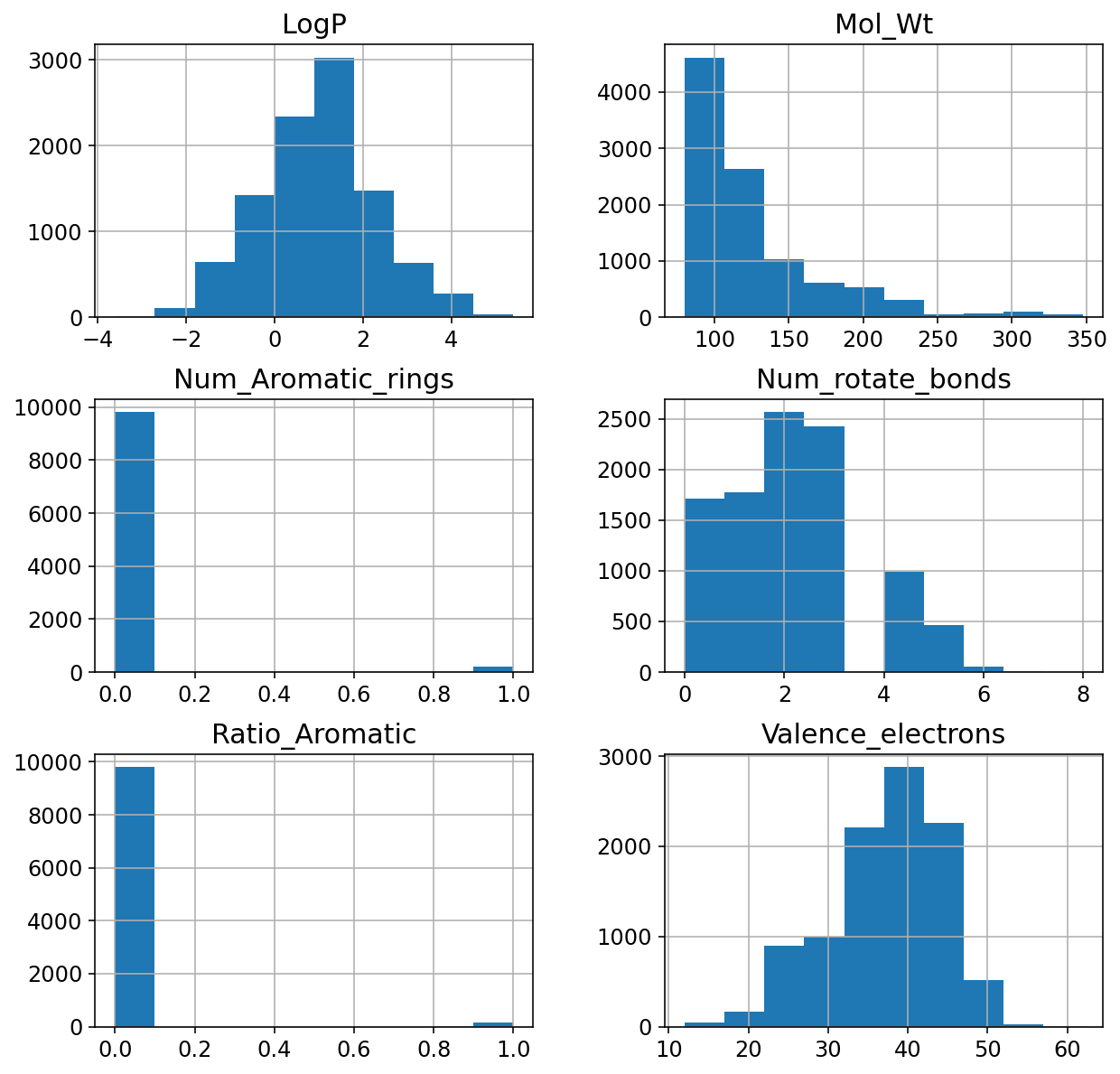
Let’s try building a model to predict a molecule’s logP value given other descriptors. We will try simple molecular descriptors and check the performance. Some molecule discriptors we will consider: 1. Molecular weight 2. Number of rotatable bonds 3. Number of aromatic compounds

logP_df.head(4)

	SMILES	LogP
0	C[C@H]([C@@H](C)Cl)Cl	2.3
1	C(C=CBr)N	0.3
2	CCC(CO)Br	1.3
3	[13CH3][13CH2][13CH2][13CH2][13CH2][13CH2]O	2.0

As before we will first convert the SMILES string into a rdkit.Chem.rdchem.Mol object, let’s write a convenience function to do so

# Getting count of aromatic elements 
_count = 0
for i in range(mol.GetNumAtoms()):
    if mol.GetAtomWithIdx(i).GetIsAromatic():
        _count = _count + 1
print(_count)

def generate_variables(smiles_list):
    
    variable_array = {'SMILES':[], 'ROMol':[], 'Mol_Wt':[],'Num_Aromatic_rings':[], 'Num_rotate_bonds':[], 'Ratio_Aromatic':[], 'Valence_electrons':[]} 
    
    for smile_entry in smiles_list: 
        mol_object = Chem.MolFromSmiles(smile_entry)
        
        mol_wt = Descriptors.MolWt(mol_object)
        mol_aromatic_rings = Descriptors.NumAromaticRings(mol_object)
        mol_rotatable_bonds = Descriptors.NumRotatableBonds(mol_object)
        
        # Calculate % of aromatic atoms in the compd
        mol_num_heavy_atom = Descriptors.HeavyAtomCount(mol_object)
        
        _count_aromatic = 0 
        for i in range(mol_object.GetNumAtoms()):
            if mol_object.GetAtomWithIdx(i).GetIsAromatic() == True:
                _count_aromatic = _count_aromatic + 1 
        
        mol_aromatic_ratio = _count_aromatic / mol_num_heavy_atom
        
        mol_val_electrons = Descriptors.NumValenceElectrons(mol_object)
        
        variable_array['SMILES'].append(smile_entry)
        variable_array['ROMol'].append(mol_object)
        variable_array['Mol_Wt'].append(mol_wt)
        variable_array['Num_Aromatic_rings'].append(mol_aromatic_rings)
        variable_array['Num_rotate_bonds'].append(mol_rotatable_bonds)
        variable_array['Ratio_Aromatic'].append(mol_aromatic_ratio)
        variable_array['Valence_electrons'].append(mol_val_electrons)
        
    return variable_array

Look at a subset from the total logP data

logP_df.shape

(14610, 2)

# Look at random 10_000 entries to keep the analysis tractable 
df_10k = logP_df.sample(10_000, random_state=42)

variable_dict = generate_variables(df_10k.SMILES)
variable_df = pd.DataFrame(variable_dict, columns=variable_dict.keys())

df_var_10k = df_10k.merge(variable_df, on='SMILES')
df_var_10k.head(2)

	SMILES	LogP	ROMol	Mol_Wt	Num_Aromatic_rings	Num_rotate_bonds	Ratio_Aromatic	Valence_electrons
0	CNCSC	0.5		91.179	0	2	0.0	32
1	CNCSC=C	1.0		103.190	0	3	0.0	36

Setup model

df_var_10k.columns

Index(['SMILES', 'LogP', 'ROMol', 'Mol_Wt', 'Num_Aromatic_rings',
       'Num_rotate_bonds', 'Ratio_Aromatic', 'Valence_electrons'],
      dtype='object')

fig, ax = plt.subplots(1,1, figsize=(10,10))
df_var_10k.hist(ax = ax);

/var/folders/_r/6hhq_8ps5118p6sqqz231j480000gq/T/ipykernel_26421/2485801931.py:2: UserWarning: To output multiple subplots, the figure containing the passed axes is being cleared
  df_var_10k.hist(ax = ax);

Split into train and validation set

from sklearn.preprocessing import StandardScaler
from sklearn.model_selection import train_test_split

df_train, df_test = train_test_split(df_var_10k, test_size=0.3, random_state=42)

print(df_train.shape, df_test.shape)

(7000, 8) (3000, 8)

Drop some columns that arent that useful for prediction

X_train = df_train.drop(columns = ['LogP','ROMol','SMILES', 'Ratio_Aromatic', 'Num_Aromatic_rings']).values
y_train = df_train.LogP.values

Pre-process input data to normalize the scale of the descriptors

# Standard Scaling X
std_scaler_X = StandardScaler()
X_train_std = std_scaler_X.fit_transform(X_train)

from sklearn.linear_model import LinearRegression

model = LinearRegression()
model.fit(X_train_std, y_train)

LinearRegression()

# predict use the trained model -- we are still using training set here 
y_pred = model.predict(X_train_std)

plt.scatter(y_train, y_pred, alpha=0.6)
plt.xlabel('True Value')
plt.ylabel('Predicted')

Text(0, 0.5, 'Predicted')

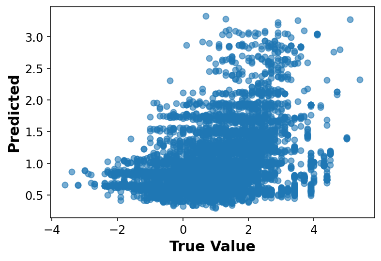
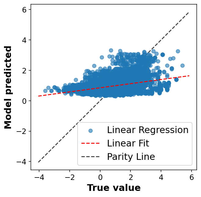
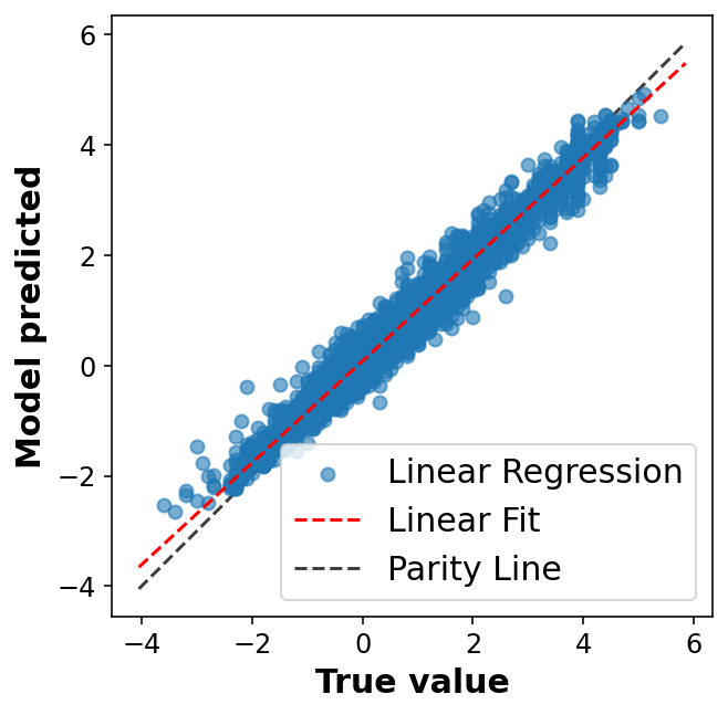
# Fancier looking plot 
fig, ax = plt.subplots(1,1, figsize=(5,5))
ax.scatter(y_train, y_pred, alpha=0.6, label='Linear Regression')

lims = [np.min([ax.get_xlim(), ax.get_ylim()]),  # min of both axes
        np.max([ax.get_xlim(), ax.get_ylim()]),  # max of both axes
        ]
# Linear fit
reg = np.polyfit(y_train, y_pred, deg=1)
ax.plot(lims, reg[0] * np.array(lims) + reg[1], 'r--', linewidth=1.5, label='Linear Fit')
ax.plot(lims, lims, 'k--', alpha=0.75, zorder=0, label='Parity Line')
ax.set_aspect('equal')
        
ax.set_xlabel('True value')
ax.set_ylabel('Model predicted')
ax.legend(loc='best');

Evaluate model success

One of the simplest ways we can evaluate the success of a linear model is using the coefficient of determination (R²) which compares the variation in y alone to the variation remaining after we fit a model. Another way of thinking about it is comparing our fit line with the model that just predicts the mean of y for any value of x.

Another common practice is to look at a plot of the residuals to evaluate our ansatz that the errors were normally distributed.

In practice, now that we have seen some results, we should move on to try and improve the model. We won’t do that here, but know that your work isn’t done after your first model (especially one as cruddy as this one). It’s only just begun!

Calculate R² using: \[R^2 =1 - \frac{\sum (y_i - \hat{y})^2}{\sum (y_i - \bar{y})^2}\]

# R2 score evaluation
SS_residuals = np.sum( (y_train - y_pred)**2 ) 
SS_total = np.sum( (y_train - np.mean(y_train))**2 )
r2 = 1 - SS_residuals / SS_total
print(r2)

0.13532814881109834

from sklearn.metrics import r2_score
print('R2 score: {}'.format(r2_score(y_train, y_pred)))

R2 score: 0.13532814881109834

Using ensemble-based model

from sklearn.ensemble import RandomForestRegressor

model = RandomForestRegressor()
model.fit(X_train_std, y_train)

RandomForestRegressor()

y_pred = model.predict(X_train_std)

# Fancier looking plot 
fig, ax = plt.subplots(1,1, figsize=(5,5))
ax.scatter(y_train, y_pred, alpha=0.6, label='Linear Regression')

lims = [np.min([ax.get_xlim(), ax.get_ylim()]),  # min of both axes
        np.max([ax.get_xlim(), ax.get_ylim()]),  # max of both axes
        ]
# Linear fit
reg = np.polyfit(y_train, y_pred, deg=1)
ax.plot(lims, reg[0] * np.array(lims) + reg[1], 'r--', linewidth=1.5, label='Linear Fit')
ax.plot(lims, lims, 'k--', alpha=0.75, zorder=0, label='Parity Line')
ax.set_aspect('equal')
        
ax.set_xlabel('True value')
ax.set_ylabel('Model predicted')
ax.legend(loc='best');

def display_performance(y_true, y_pred):
    from sklearn.metrics import r2_score, mean_absolute_error, mean_squared_error
    r2 = r2_score(y_true, y_pred)
    mae = mean_absolute_error(y_true, y_pred)
    rmse = np.sqrt(mean_squared_error(y_true, y_pred))
    
    print('R2: {0:0.2f}\n'
          'MAE: {1:0.2f}\n'
          'RMSE: {2:0.2f}'.format(r2, mae, rmse))
    return(r2, mae, rmse)

display_performance(y_train,y_pred);

R2: 0.91
MAE: 0.29
RMSE: 0.40

Fingerprints

Compress molecules into vectors for mathetical operations and comparisons. First we will look at MorganFingerprint method. For this method we have to define the radius and the size of the vector being used.

More information on different Circular Fingerprints can be read at this blogpost. Highly recommended

Presentation by Gregory Landrum (creator of RDkit) on Fingerprints
RDkit Blog entry of visualizing the fingerprint bitvectors. Using the new fingerprint bit rendering code

# Fingerprints
from rdkit.Chem import AllChem

radius = 2 # How far from the center node should we look at? 
ecfp_power = 10 # Size of the fingerprint vectors  
ECFP = [ np.array(AllChem.GetMorganFingerprintAsBitVect(m, radius, nBits = 2**ecfp_power)) for m in df_train['ROMol'] ]

len(ECFP)

df_train['ECFP'] = ECFP

df_train.sample(2)

	SMILES	LogP	ROMol	Mol_Wt	Num_Aromatic_rings	Num_rotate_bonds	Ratio_Aromatic	Valence_electrons	ECFP
6160	C[NH+](C)CCl	1.0		94.565	0	1	0.0	32	[0, 0, 0, 0, 0, 0, 0, 0, 0, 0, 0, 0, 0, 0, 0, ...
1564	CCCNCO	0.1		89.138	0	3	0.0	38	[0, 0, 0, 0, 0, 0, 0, 0, 0, 0, 0, 0, 0, 0, 0, ...

X_train = df_train.ECFP.values
X_train = np.stack(X_train, axis=0)

y_train = df_train.LogP.values

# Standard Scaling
std_scaler = StandardScaler()
X_train_std = std_scaler.fit_transform(X_train)

model = RandomForestRegressor()
model.fit(X_train_std, y_train)

RandomForestRegressor()

y_pred = model.predict(X_train_std)

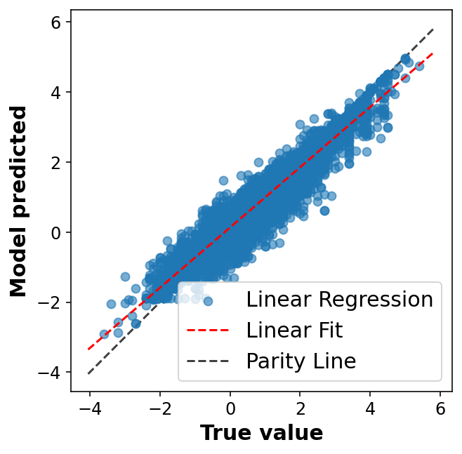
# Fancier looking plot 
fig, ax = plt.subplots(1,1, figsize=(5,5))
ax.scatter(y_train, y_pred, alpha=0.6, label='Linear Regression')

lims = [np.min([ax.get_xlim(), ax.get_ylim()]),  # min of both axes
        np.max([ax.get_xlim(), ax.get_ylim()]),  # max of both axes
        ]
# Linear fit
reg = np.polyfit(y_train, y_pred, deg=1)
ax.plot(lims, reg[0] * np.array(lims) + reg[1], 'r--', linewidth=1.5, label='Linear Fit')
ax.plot(lims, lims, 'k--', alpha=0.75, zorder=0, label='Parity Line')
ax.set_aspect('equal')
        
ax.set_xlabel('True value')
ax.set_ylabel('Model predicted')
ax.legend(loc='best');

display_performance(y_train,y_pred);

R2: 0.97
MAE: 0.15
RMSE: 0.22

Similarity

RDKit provides tools for different kinds of similarity search, including Tanimoto, Dice, Cosine, Sokal, Russel… and more. Tanimoto is a very widely use similarity search metric because it incorporates substructure matching. Here is an example

ref_mol = df_var_10k.iloc[4234]['ROMol']

ref_mol

# Generate finger print based representation for that molecule 
ref_ECFP4_fps = AllChem.GetMorganFingerprintAsBitVect(ref_mol, radius=2)

df_var_10k_ECFP4_fps = [AllChem.GetMorganFingerprintAsBitVect(x,2) for x in df_var_10k['ROMol']]

Estimate the similarity of the molecules in the dataset to the reference dataset, there are multiple ways of doing it: we are using Tanimoto fingerprints

from rdkit import DataStructs
similarity_efcp4 = [DataStructs.FingerprintSimilarity(ref_ECFP4_fps, x) for x in df_var_10k_ECFP4_fps]

df_var_10k['Tanimoto_Similarity (ECFP4)'] = similarity_efcp4
df_var_10k['Tanimoto_Similarity (ECFP4)'] = df_var_10k['Tanimoto_Similarity (ECFP4)'].round(3)
PandasTools.FrameToGridImage(df_var_10k[:10], legendsCol="Tanimoto_Similarity (ECFP4)", molsPerRow=4)

Sorting the molecule similarity for clarity:

df_var_10k = df_var_10k.sort_values(['Tanimoto_Similarity (ECFP4)'], ascending=False)
PandasTools.FrameToGridImage(df_var_10k[:10], legendsCol="Tanimoto_Similarity (ECFP4)", molsPerRow=4)